IsoAxis

1. Introduction.

1.1. Objectives.

The objective of this project is to generate a computer animation of an IsoAxis (described in the following section) as an example of the kinematic animation of a mechanical system featuring multiple constraints among its component elements and several degrees of freedom.

1.2. System Description.

The IsoAxis (US Patent No. 3302321) was discovered by Wallace Walker in 1958 while working on a project aimed at achieving structural configurations for paper.

It consists of a two-dimensional state of paper folded into a grid of sixty isosceles right triangles, forming a three-dimensional ring that can rotate around its center upon itself, yielding a cycle of curious-looking configurations.

Figure 1: Net development and perspective view of an IsoAxis

2. Analytical Approach.

2.1. System Definition.

As shown in Figure 1, the system is composed of six sectors with ten triangles each, arranged at 60° intervals to form a ring structure [1].

The first necessary step to obtain a kinematic description of the IsoAxis is determining its number of degrees of freedom. To do this, we will consider an arbitrary vertex of the sector shown in Figure 2; for instance, vertex 0. The position of this point in space is fixed by 3 coordinates. From this point, the position of an adjacent vertex (5) can be determined using two additional coordinates (for example, two angular coordinates). The two points defined in this manner determine a straight line; with the help of another coordinate, the position of the vertex that closes the triangle (1) can be obtained. Following this line of reasoning for vertices 1 to 6 (vertices 7, 8, and 9 are obtained by symmetry), we conclude that 10 coordinates are required to define the position of all vertices.

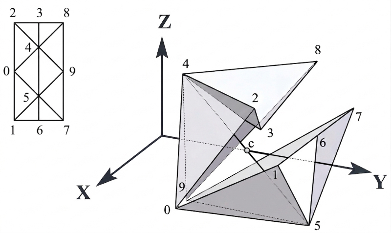
Figure 2: IsoAxis Sector

However, if we introduce the necessary constraints so that the sector can form part of a ring (vertices 0, 1, and 2 must lie on the plane $x=\sqrt{3}y$ ; and vertices 3 to 6 must lie on the plane x=0), we obtain 7 equations, reducing the number of degrees of freedom to 3. Fixing the height of the sector along the Z-axis (in Figure 3, by positioning the center of segment (4 5) on the Y-axis) leaves a total of 2 degrees of freedom.

Defining the angles $\alpha ,\beta ,\gamma ,\delta$ as shown in Figure 3:

$$\alpha =\frac{1}{2}\angle \left(9c0\right)$$

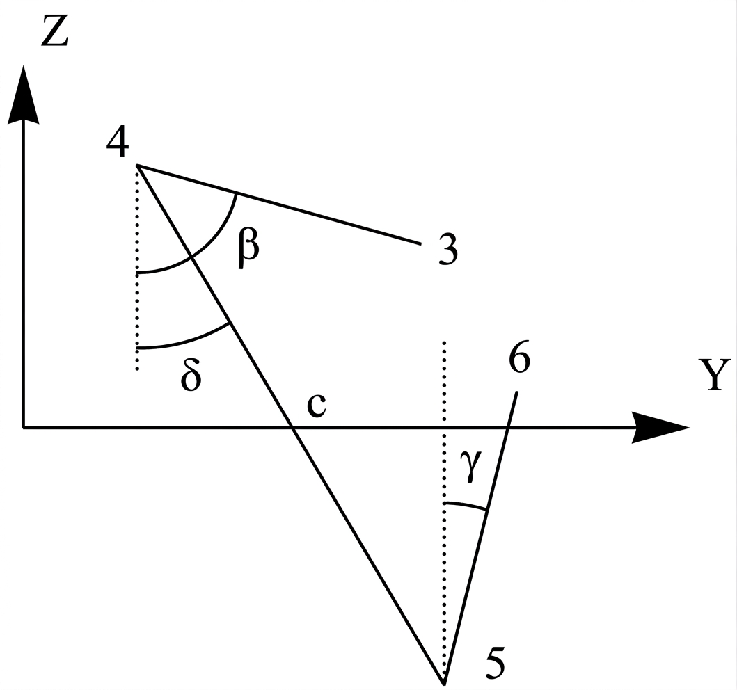
Figure 3: Definition of angular coordinates

we can choose $\delta and\alpha$ as the degrees of freedom, meaning the rotation of the IsoAxis will be directly coupled to the variable $\delta$ .

Consequently, the coordinates of vertices 0 to 6 are given by:

• $$p_0=(sen\alpha ,\sqrt{3}sen\alpha ,-cos\alpha sen\delta )$$
• $$p_1=(\frac{y_1}{\sqrt{3}},y_1,z_1)$$
• $$p_2=(\frac{y_2}{\sqrt{3}},y_2,z_2)$$
• $$p_3=(0,\sqrt{3}sen\alpha +cos\delta cos\alpha -sen\delta +sen\beta ,cos\delta -cos\beta )$$
• $$p_4=(0,\sqrt{3}sen\alpha +cos\delta cos\alpha -sen\delta ,cos\delta )$$
• $$p_5=(0,\sqrt{3}sen\alpha +cos\delta cos\alpha +sen\delta ,-cos\delta )$$
• $$p_6=(0,\sqrt{3}sen\alpha +cos\delta cos\alpha +sen\delta +sen\gamma ,-cos\delta +cos\gamma )$$

where six unknowns appear: $y_1,z_1,y_2,z_2,\beta ,\gamma$ .

These variables can be calculated analytically using the equations derived from the conditions of perpendicularity between segments and distances between points.

2.2. Mathematical Solution.

Note: [n m] denotes the segment connecting vertices n and m; and |[n m]| denotes the length of that segment.

First, vertex 1 must be computed using the following equations:

1. $$\overrightarrow{p_0{p}_5}·\overrightarrow{p_1{p}_5}=0$$
2. $$\left|\overrightarrow{p_1{p}_5}\right|=\sqrt{2}$$

Expanding these terms:

3. $$y_1(\frac{x_0}{\sqrt{3}}+y_0-y_5)+z_1(z_0-z_5)=y_5(y_0-y_5)+z_5(z_0-z_5)$$
4. $${\left(\frac{y_1}{\sqrt{3}}\right)}^2+{(y_1-y_5)}^2+{(z_1-z_5)}^2=2$$

This system yields two solutions for $(y_1,z_1)$; we select the one that minimizes the angle $\widehat{c{p}_5{p}_1}$ .

For the case where $z_0=z_5$ :

$$\begin{array}{l}{y}_1=\frac{y_5(y_0-y_5)}{\frac{x_0}{\sqrt{3}}+y_0-y_5}\\ x_1=\frac{y_1}{\sqrt{3}}\\ z_1=z_5\pm \sqrt{2-x_1^2-{(y_1-y_5)}^2}\end{array}$$

Otherwise, the system can be expressed as:

5. $$a{y}_1+z_1=b$$
6. $${\left(\frac{y_1}{\sqrt{3}}\right)}^2+{(y_0-u)}^2+{(z_1-v)}^2=2$$

where
$$a=\frac{\frac{x_0}{\sqrt{3}}+y_0-y_5}{z_0-z_5}$$ $$b=z_5+\frac{y_0-y_5}{z_0-z_5}$$ $$u=y_5$$ $$v=z_5$$

making it possible to solve for $y_1$ in terms of $(a,b,u,v)$, yielding:

Once the coordinates of vertex 1 are determined, it is possible to compute the position of vertex 6 using the perpendicularity condition:

from which we obtain:

There are two distinct solutions for $\gamma$; we select the one that minimizes the angle $\widehat{p_4{p}_5{p}_6}$ .

The calculation for vertex 2 is analogous to that of vertex 1, substituting vertex 5 with vertex 4.

The calculation for vertex 3 is analogous to that of vertex 6:

With this, the spatial positions of all vertices are fully determined as a function of $\delta$ and $\alpha$ .

2.3. Boundary Constraints.

Up to this point, the coordinates of the vertices have been calculated without factoring in a series of physical constraints that limit the valid range of the angle alpha for each given value of delta.

These geometric constraints arise, on one hand, from the impenetrability of the sector faces, and on the other, from the mathematical requirement for valid real solutions to exist within the quadratic equations formulated in the previous section [2].

Some of these boundary constraints can be easily defined and solved analytically, whereas others must be resolved using numerical methods.

Figure 4: Kinematic constraints for the variable alpha

For $y_4\ge 0$, based on the geometric expression of $p_4$, the governing equation takes the form:

where:

which provides a direct analytical solution.

The analytical solution for ${\mathrm{y<!--="5"-->5<mo>\ge </mo><mn>0</mn>}}_{}$ is perfectly analogous; whereas for $y_5\le 2$ the system structure remains identical with coefficients:

Through these equations, the permissible range of variation for $\alpha$ can be confined to a relatively narrow band (note that values corresponding to the upper boundary region of the solution for $y_5\le 2$ can yield mathematically valid configurations, but they lack geometric continuity with the sequence that constitutes the standard motion cycle of the IsoAxis).

However, the analytical solution of the constraints associated with the existence of real roots in the second-degree equations must be performed using numerical methods. The main computational challenges encountered are the exceptionally narrow margin of variation for $\alpha$ in specific operational zones and the appearance of clearly perceivable numerical oscillations across several variables resulting from minute fluctuations in the angle $\alpha$.

In fact, in the operational zone corresponding to values of $\delta$ approaching $\pi /2$, a valid solution for the angle $\gamma$ can only be achieved if the coordinate $y_4$ is allowed to take a value slightly below zero (which physically corresponds to accepting elastic deformations within a “real” material model). Figure 5 illustrates the evolution of several significant variables of the system as a function of $\delta$.

The values of ${\gamma }_1$ and ${\gamma }_2$ correspond to the values of the vertex angle $\angle \left(456\right)$, expressed in radians, for the two possible mathematical solutions of $\gamma$.

Figure 5: System Kinematic Evolution

Note that variables $y_5$, $y_4$, and $y_1$ drop slightly below zero at certain configuration states; in a perfectly rigid structure, these values must remain strictly positive, which implies that the only viable physical solution is to allow for micro-deformations within the mechanism.

3. Computer Animation.

To visualize the mechanical model, three software applications were developed between 1991 and 1994. One implemented the RenderMan interface, enabling rendering capabilities on any workstation; another was built using HP's Starbase graphics library; and the final version utilized Silicon Graphics' GL native library, which enabled real-time 3D animation on hardware specifically optimized for spatial calculations.

The original animation was produced in 1993 using the RenderMan system running on MacOS.

Figure 6: Animation Clip (QuickTime format, 1.2 MB)
Also available in MPG format, 1.2 MB (compressed quality)
Also available in AVI/DivX format, 0.5 MB

4. Source Code and Executables.

The complete source code, which relies on OpenGL, GLUT, and libjpeg libraries, can be obtained at:

• ftp://ivo.cps.unizar.es/pub/SPDsoft/isoaxis/isoaxis-1.0.tar.gz

• macOS Sierra
• MacOS X 10.2.x
• MacOS 9.x
• IRIX 6.x
• Linux 2.4.x x86
• Solaris 7 SPARC
• Solaris 2.5 SPARC
• Tru64 5.x
• HP-UX 11.x
• Windows 98/ME/NT/2000/XP

Regardless of the pre-built platforms listed, compiling the project should be straightforward on any modern platform supporting the GLUT API.

Note: Some of these legacy binaries may be dynamically linked against specific OpenGL, GLUT, and/or jpeg shared libraries. If a binary fails to execute on your system, you will need to locate and install the missing runtime dependencies.

Note: Parts of this codebase were authored many years ago and lack modern refactoring standards, meaning it should not be referenced as an optimal coding layout.

5. External Links.

From "une balade dans le monde des polyèdres", by Maurice Starck:

• The kaleidohedron from the IsoAxis grid

[1] This theoretical framework assumes a geometric symmetry that may not necessarily manifest in real-world physical models. However, the normal inversion cycle of the IsoAxis® is inherently symmetric, and analyzing 1/6th of the complete ring presents an analytical problem that is already sufficiently complex on its own.

[2] Note: As shown in the constraint plots, there is an operational region around a delta of 90° where the boundary curves y5=0 and y4=0 converge toward a single unique solution for alpha. In practice, this point solution violates additional non-analytical constraints, indicating that an ideal kinematic motion sequence without any material deformation is geometrically impossible.

Analytical study conducted in 1991 by spd@daphne.cps.unizar.es